Intuition and/or visualisation of Ito integral/Ito's lemma
I find the intuitive explanation by Paul Wilmott particularly appealing.
Fix a small $h>0$. The stochastic integral $$\int_0^{h} f(W(t))\ dW(t)=\lim\limits_{N\to\infty}\sum\limits_{j=1}^{N} f\left(W(t_{j-1})\right)\left(W(t_{j})-W({t_{j-1}})\right),\quad t_j= h\frac{j}{N},$$ involves adding up an infinite number of random variables. Let's substitute every term $f\left(W(t_{j-1})\right)$ with its formal Taylor expansion. Then there are several contributions to the sum: those that are a sum of random variables and those that are a sum of the squares of random variables, and then there are higher-order terms.
Add up a large number of independent random variables and the Central Limit Theorem kicks in, the end result being a normally distributed random variable. Let's calculate its mean and standard deviation.
When we add up $N$ terms that are normal, each with a mean of $0$ and a standard deviation of $\sqrt{h/N}$, we end up with another normal, with a mean of $0$ and a standard deviation of $\sqrt{h}$. This is our $dW$. Notice how the $N$ disappears in the limit.
Now, if we add up the $N$ squares of the same normal terms then we get something which is normally distributed with a mean of $$N\left(\sqrt{\frac{h}{N}}\right)^2=h$$ and a standard deviation which is $h\sqrt{2/N}.$ This tends to zero as $N$ gets larger. In this limit we end up with, in a sense, our $dW^2(t)=dt$, because the randomness as measured by the standard deviation disappears leaving us just with the mean $dt$.
The higher-order terms have means and standard deviations that are too small, disappearing rapidly in the limit as $N\to\infty$.
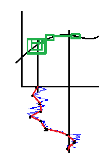
I know this thread is already two years old, but, while preparing for a path integration exam, I arrived at an intuitive picture that sheds some light on the origin of the extra term. The picture represents an integral of a smooth function with respect to a concrete realization of Brownian motion. The sum of the areas of the green rectangles represents the difference between Ito (using the left point of each interval) and "anti-Ito" (using the right point of each interval) for sampling of the Brownian motion represented by the red line. Finer sampling leads to smaller rectangles, but they overlap more and more (because Brownian motion is not monotonic), so even if the area occupied by them tends to zero, the sum of their areas does not. This suggests (only suggests -- it is an upper bound on the difference, not a lower bound) that there is a "room" for Ito and "anti-Ito" to differ in their values. Stratonovich can be expected to lie somewhere in between.
Look at the following image:
https://lh6.googleusercontent.com/-bEPzm01WyGk/T-WplGQAc3I/AAAAAAAAACQ/mZr-5p0VUrw/s317/integral-wrt-brownian-motion.png
Robert Anderson used nonstandard analysis to generate Brownian motion from a finite random walk obtained from coin tosses, where "finite" means indexed by an infinite, non-standard natural number. The corresponding random walk has bounded variation under a non-standard bound. One can then do everything in terms such an random walk, as has been done without rigorous justification before. The Itô-integral can be obtained from a Stiltjes-integral on the random walk, they differ only by an infinitesimal. An outline of the arguments can be found here. For the details, see:
MR0464380 (57 #4311) Anderson, Robert M. A non-standard representation for Brownian motion and Itô integration. Israel J. Math. 25 (1976), no. 1-2, 15--46.